Static Single Assignment Algorithm for MLIR

In this post we will talk about the algorithm used in Kunai for generating the SSA form in the Dialect created with MLIR for Dalvik Bytecode analysis, MjolnIR.

Authors

• Aymar Cublier
• Eduardo Blázquez

Few notes on Static Single Assignment (SSA)

As stated in 1, SSA was conceived to make program analyses more efficient by compactly representing use-def chains. Since the main property of SSA form is that variables are defined just once, a definition is just a single point, so a definition can be stored as a pointer to an IR instruction. And uses of that value, can be defined as a list of pointers. In other case, we should keep track of where a variable is defined, since multiple definitions exist.

One of the first algorithms for generating SSA (and the first used on Kunai 4) was Cytron et al.’s algorithm, which guarantees a form of minimality on the number of phi function placed. The problem with this algorithm is that it relies on a program represented as a Control Flow Graph (CFG), and things like the dominance tree and dominance frontiers for placing the phi functions. After that, liveness analyses or dead code elimination are performed for removing unnecessary phi functions. So in that case we will have to follow the next step:

1. Representing input as a CFG.
2. Computing Dominance Tree and Dominance frontiers.
3. Placing Phi functions.
4. Applying renaming of variables.

In our case, the IR will be used for representing Dalvik Bytecode, and while we already have a disassembled bytecode in a CFG, it would be costly to compute the Dominance Tree and Dominance frontiers, also we want to directly emit IR based on MLIR. In the next sections we explore the algorithm used based in the algorithm given by 1 and the explanations from 3.

Algorithm Explanation

Since the MLIR framework does not consider phi instructions, MLIR blocks can have parameters. In case a value cannot be retrieved in a basic block (through local value numbering), we look for it in its predecessor blocks. We set the value we need in the block as ‘required for the block’.

The value is searched in the block’s predecessor, but if the value we are looking for is not in the predecessor block either, we set that value for that predecessor as ‘required’ too, and in a recursive way that value will have to be searched in its own predecessors.

We then have two main functions: one is readLocalVariable, that looks for the Value in the current block applying the theory behind local value numbering, the other is readLocalRecursiveVariable and is used in the case we need to look for the Value in previous blocks,and then apply the global value numbering in the graph.

Issue with MLIR

The previous algorithm is very well explained in 1, also we can find an explanation of phi functions placement in order to avoid infinite recursion. The main difference between the algorithm they explain, and the one we use is that in MLIR as explained at the beginning of this section, we do not have phi functions, we have basic block parameters, and its construction design needs from a previous analysis. In the same way we add these values as basic block parameters in the block that ‘required’ the value, we will have to make the terminator instruction from a predecessor to ‘send’ as the value as one of its parameter. But while it is easy to add a parameter in a block, it is not that easy to add the parameters in the terminal instructions. Therefore, we need to apply the Data Flow Analysis before creating the terminal instructions.

We use a structure like the following one to keep track of the values during the Data Flow Analysis:

type edge_t = pair<BasicBlock, BasicBlock>;

struct BasicBlockDef
{
    /// Map a register to its definition in IR
    Map<reg, Value> Defs;
    /// required values from the basic block
    set<reg> required;
    /// keep track of values that will be "send"
    /// to next basic blocks
    Map<edge_t, Vector<Value>> jmpParameters;    

    /// Block is sealed, means no more predecessors will be
    /// added nor analyzed.
    bool Analyzed;

    BasicBlockDef() : Analyzed(False) {}
};

We additionally have a map like the following to keep this structure for each basic block:

Map<BasicBlock, BasicBlockDef> CurrentDef;

Data Flow Analysis

Our algorithm first goes over each basic block, generating each instruction, but avoiding generating terminal instructions (e.g. jumps, conditional jumps, switch). During the generation of instructions, we apply the Data Flow Analysis.

Whenever we generate a new value, we apply local value numbering for keeping track of last value for each register used in a block. For doing that, we will have the next function (same function to the one presented at 1):

writeLocalVariable(BB, Reg, Value):
    CurrentDef|BB|.Defs|Reg| = Val

With this, we store the last value assigned for a register in a basic block. Now when a value is needed, we look for it first in the current block, and in case the value is not defined in this block, we look for it in its predecessor blocks.

In case we look for it in our block, we use the following function:

readLocalVariable(BB, Reg):
    Val = CurrentDef|BB|.Defs.get(Reg)
    if Val:
        return Val
    return readLocalVariableRecursive(BB, Reg)

This function will try to obtain the definition of the value in the current block, but in case the value was not defined in the current block, we have to look for it in its predecessors, and for doing that we have the call to the function in the last line.

In order to look in the predecessors, we apply the following algorithm:

• Insert the searched Reg into the list of required values in current block.
• Look for that Reg in the predecessor blocks of the current block
• As we are generating the SSA form at the moment, we have to check if the previous block was already analyzed (e.g. in a loop we could have the body was not analyzed yet). In case it was not, generate that block.
• Look for the value in the predecessor using readLocalVariable.
• Once the value is found, in case it is in the required list, add it as a parameter to the basic block and remove it from the required list.
• Keep track of the value for generating the terminal instructions after generating the CFG. In order to do that, keep the value in a map which key is an edge between predecessor block and current block.

We can find the code in the following snippet:

readLocalVariableRecursive(BB, Reg)
    new_value : Value

    /// add to Reg to required
    CurrentDef|BB|.required.insert(Reg)

    for pred in predecessors(BB):
        if not CurrentDef|pred|.Analyzed:
            gen_block(pred)
        Val = readLocalVariable(pred, Reg)

        /// If the value is required, add argument to the block
        /// write the local variable and erase from required
        if CurrentDef|BB|.required.contains(Reg):
            /// create value as argument in block
            new_value = BB.addArgument(Val)
            /// write variable as local in basic block
            writeLocalVariable(BB, Reg, new_value)
            /// remove from required
            CurrentDef|BB|.required.erase(Reg)
        
        /// now add the Value as a jump argument for later
        /// when we generate terminator instructions
        CurrentDef|pred|.jmpParameters|<pred,BB>|.back(Val)
    
    return new_value

Once we have finished generating the CFG, we can start generating the terminal instruction for each basic block, and because we have already cached the necessary parameters, we are able to generate the different terminal instructions with its parameters.

Representation

For making easier to understand the problem and the algorithm, we have represented the cases in a few scenarios. We start with the simples case where we apply local value numbering, where we have a definition of a local value, and an instruction requiring using that same value in the same block (in the figures, the registers from the bytecode will be represented as vX and the values as %X, these values are not a one to one representation of the registers).

Local Value Numbering.

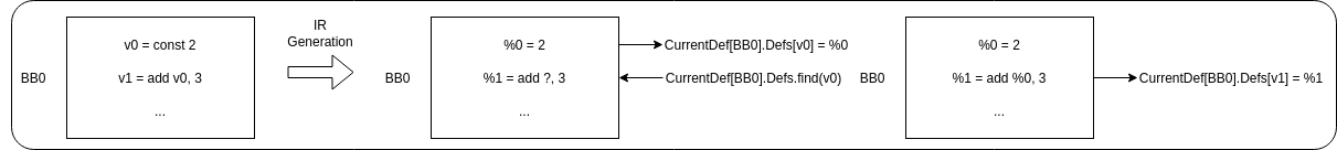
In this case, the first instruction defined the value %0 in the IR, and store it as a definition for v0 register. The next instruction uses the register v0, so we need to look for the value defined for that register. Luckily in this case, the value has been previously defined in the same block, so calling to readLocalVariable, we obtain the defined value.

The next case is the simplest case of global value numbering, in the case we only have one predecessor, and the value we need was previously defined by that predecessor:

Global Value Numbering Simple Case.

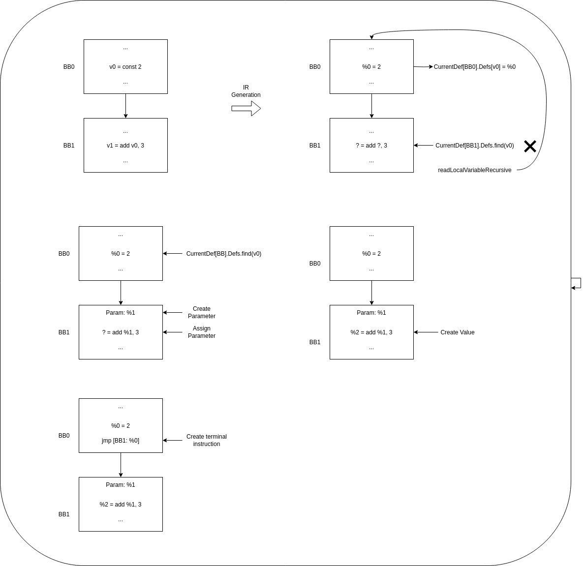
In this case, when the algorithm tries to obtain the definition of the needed value in the current basic block it fails, and have to call to readLocalVariableRecursive. In this case, we find that the value was defined in the previous block, then it is possible to create the parameter and assign it to the instruction, and record the value for the moment when we generate the terminal instructions, that will be once we have transformed all basic blocks to our MLIR Dialect.

Now we will see a more complicated case. In this case, our immediate predecessor has not defined the required value, so it will have to look for the value on its own predecessor, this value will have to be propagated through basic block parameters and through terminal instructions.

Global Value Numbering Complicated Case.

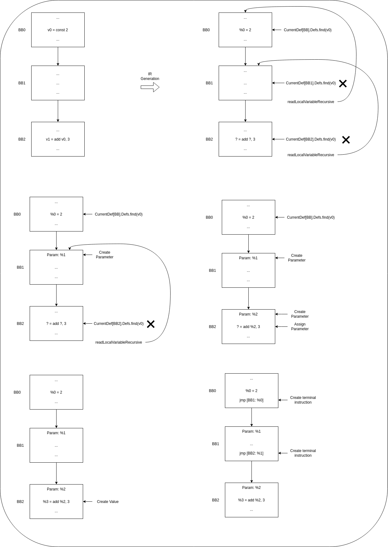
The process is similar to the simplest case, but because the value is not found in the predecessor, the predecessor block will have to set the Reg as ‘required’, and look for its value on its predecessor. Once we find it, the recursion stops and the algorithm starts propagating the value through the block parameters, and keeping track of them for later generating the terminal instructions.

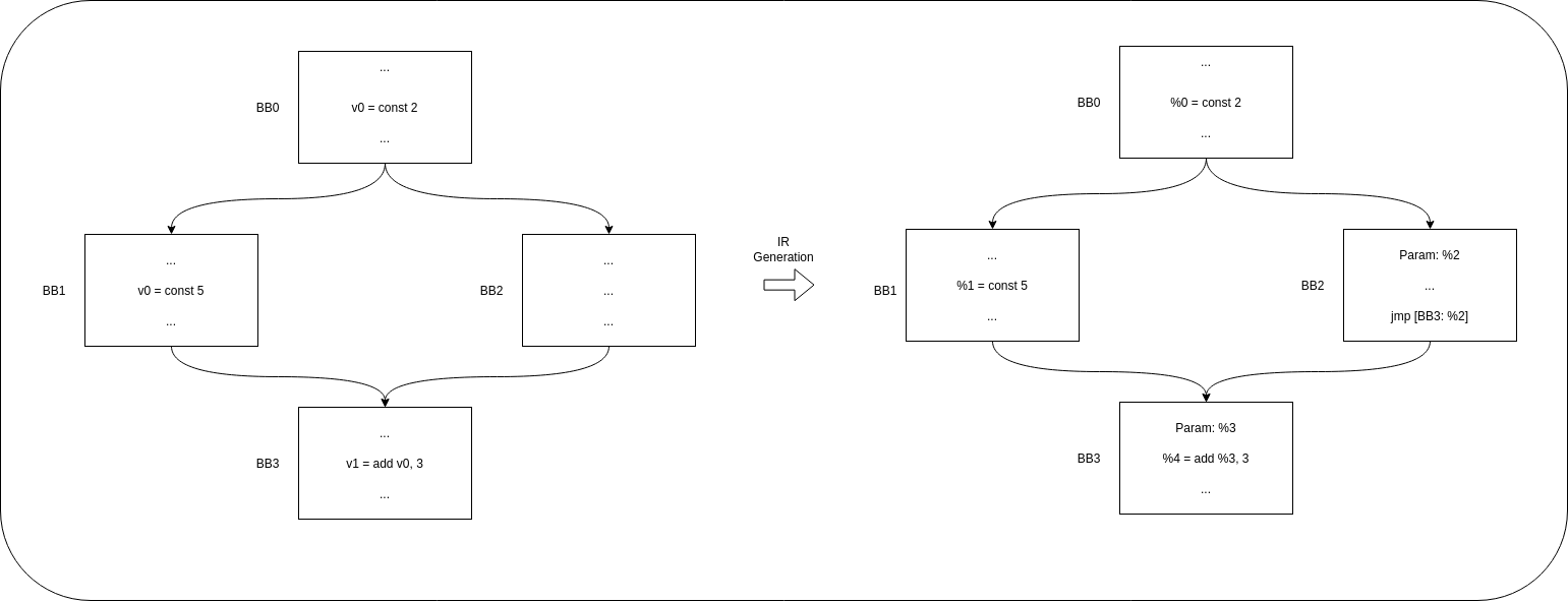
The next two figures represent two use cases, one is an if-else example where we can see that since the algorithm looks for the value in all the predecessors from a basic block, in the predecessor where the value is not defined, this will have to be propagated from previous basic blocks, allowing to retrieve all the possible previous values.

If-Else Example.

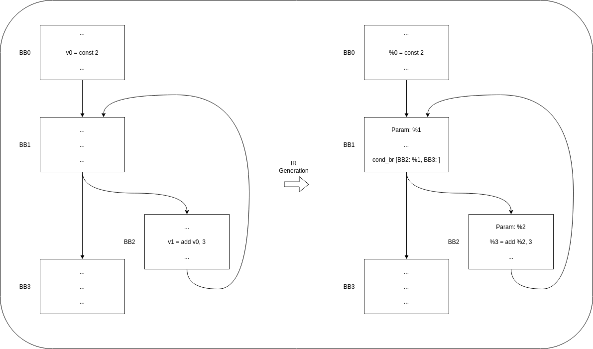
The other example we find is the next, a loop where we could find that the body of the loop requires a value that was not defined by the predecessor. In this case, the predecessor (BB1 in this case) will look for the value first on BB0, since looking for the value in its other predecessor (BB2) would create an infinite recursion problem. Since the value is propagated and created as a basic block parameter in BB1, BB2 will obtain a correct value and infinite recursion is stopped here.

Loop Example.

Clarification

We will like to clarify that in this case, the algorithm is not applied to a source code, but to a disassembled code from Dalvik Bytecode, so we do not have access to things like loop headers or loop bodies, nor similar structures. All we access is a CFG from the disassembled output from Dalvik bytecode.

You can find all the code of the algorithm at 5 and 6.

Acknowledgments

We would like to thank Alex Denisov for his explanation about the algorithm used at 3, that were really useful for writing the one used in Kunai. Also MLIR community for helping us with few comments on compilation errors on our MLIR Dialect.

References

• 1: Simple and Efficient Construction of Static Single Assignment Form
• 2: Value Numbering
• 3: Compiling Ruby. Part 3: MLIR and compilation
• 4: Cytron Algorithm Kunai
• 5: MjolnIR Lifter header
• 6: MjolnIR Lifter source code